Grading Eye Inflammation
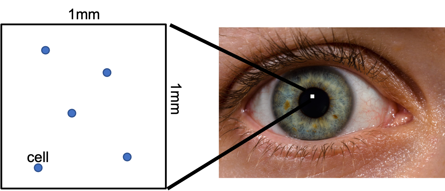
When a patient has eye inflammation, eye doctors "grade" the inflammation. When "grading" inflammation they randomly look at a single 1 millimeter by 1 millimeter square in the patient's eye and count how many "cells" they see.
There is uncertainty in these counts. If the true average number of cells for a given patient's eye is 6, the doctor could get a different count (say 4, or 5, or 7) just by chance. As of 2021, modern eye medicine does not have a sense of uncertainty for their inflammation grades! In this problem we are going to change that. At the same time we are going to learn about Poisson distributions over space.
Why is the number of cells observed in a 1x1 square governed by a Poisson process?
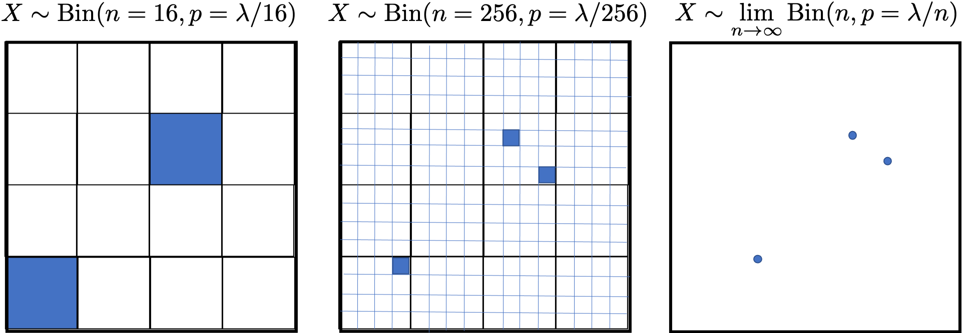
We can approximate a distribution for the count by discretizing the square into a fixed number of equal sized buckets. Each bucket either has a cell or not. Therefore, the count of cells in the 1x1 square is a sum of Bernoulli random variables with equal $p$, and as such can be modeled as a binomial random variable. This is an approximation because it doesn't allow for two cells in one bucket. Just like with time, if we make the size of each bucket infinitely small, this limitation goes away and we converge on the true distribution of counts. The binomial in the limit, i.e. a binomial as $n \rightarrow \infty$, is truly represented by a Poisson random variable. In this context, $\lambda$ represents the average number of cells per 1$\times$1 sample. See Figure 2.
For a given patient the true average rate of cells is 5 cells per 1x1 sample. What is the probability that in a single 1x1 sample the doctor counts 4 cells?
Let $X$ denote the number of cells in the 1x1 sample. We note that $X \sim \Poi(5)$. We want to find $P(X=4)$.
\[P(X=4) = \frac{5^4 e^{-5}}{4!} \approx 0.175\]
Multiple Observations
For a given patient the true average rate of cells is 5 cells per 1mm by 1mm sample. In an attempt to be more precise, the doctor counts cells in two different, larger 2mm by 2mm samples. Assume that the occurrences of cells in one 2mm by 2mm samples are independent of the occurrences in any other 2mm by 2mm samples. What is the probability that she counts 20 cells in the first samples and 20 cells in the second?
Let $Y_1$ and $Y_2$ denote the number of cells in each of the 2x2 samples. Since there are 5 cells in a 1x1 sample, there are 20 samples in a 2x2 sample since the area quadrupled, so we have that $Y_1 \sim \Poi(20)$ and $Y_2 \sim \Poi(20)$. We want to find $P(Y_1 = 20 \land Y_2 = 20)$. Since the number of cells in the two samples are independent, this is equivalent to finding $\P(Y_1 = 20) \P(Y_2=20)$.
Estimating Lambda
Inflammation prior: Based on millions of historical patients, doctors have learned that the prior probability density function of true rate of cells is:
\begin{align*}
f(\lambda) = K \cdot \lambda \cdot e ^{-\frac{\lambda}{2}}
\end{align*}
Where $K$ is a normalization constant and $\lambda$ must be greater than 0.
A doctor takes a single sample and counts 4 cells. Give an equation for the updated probability density of $\lambda$. Use the "Inflammation prior" as the prior probability density over values of $\lambda$. Your probability density may have a constant term.
Let $\theta$ be the random variable for true rate. Let $X$ be the random variable for the count
\begin{align*}
f(\theta = \lambda | X = 4)
&= \frac{P(X=4|\theta = \lambda) f(\theta = \lambda)}{P(X = 4)} \\
&= \frac{\frac{\lambda^{4} e^{-\lambda}}{4!} \cdot K \cdot \lambda \cdot e^{\lambda / 2}}{P(X = 4)} \\
&= \frac{K \cdot \lambda^5 e^{-\frac{3}{2}\lambda}}{4! P(X=4)}
\end{align*}
A doctor takes a single sample and counts 4 cells. What is the Maximum A Posteriori estimate of $\lambda$?
Maximize the "posterior" of the parameter calculated in the previous section:
\begin{align*}
\argmax_\limits\lambda \frac{K \cdot \lambda^5 e^{-\frac{3}{2}\lambda}}{4! P(X=4)}
&= \argmax_\limits\lambda \lambda^5 e^{-\frac{3}{2}\lambda} \\
\end{align*}
Take logarithm (preserves argmax, and easier derivative):
\begin{align*}
&= \argmax_\limits\lambda \log \left(\lambda^5 e^{-\frac{3}{2}\lambda} \right) \\
&= \argmax_\limits\lambda \left(5 \log \lambda -\frac{3}{2}\lambda\right)
\end{align*}
Calculate the derivative with respect to the parameter, and set equal to 0
\begin{align*}
0 &= \frac{\partial}{\partial \lambda} \left(5 \log \lambda -\frac{3}{2}\lambda\right) \\
0 &= \frac{5}{\lambda} -\frac{3}{2} \\
\lambda &= \frac{10}{3}
\end{align*}
Explain, in words, the difference between the two estimates of lambda in the two previous parts.
The estimate in the first part is a ``distribution" (also called a soft estimate) whereas the estimate in the second part is a single value (also called a point estimate). The former contains information about confidence.
What is the MLE estimate of $\lambda$?
The MLE estimate doesn't use the prior belief. The MLE estimate for a poisson is simply the average of the observations. In this case the average of our single observation is 4. MLE is not a great tool for estimating our parameter from just one datapoint.
A patient comes on two separate days. The first day the doctor counts 5 cells, the second day the doctor counts 4 cells. Based only on this observation, and treating the true rates on the two days as independent, what is the probability that the patient's inflammation has gotten better (in other words, that their $\lambda$ has decreased)?
Let $\theta_1$ be the random variable for lambda on the first day and $\theta_2$ be the random variable for lambda on the second day.
\begin{align*}
f(\theta_1 = \lambda | X = 5) &= K_1 \cdot \lambda^6 e^{-\frac{3}{2}\lambda} \\
f(\theta_2 = \lambda | X = 4) &= K_2 \cdot \lambda^5 e^{-\frac{3}{2}\lambda}
\end{align*}
The question is asking what is $P(\theta_1 > \theta_2)$? There are a few ways to calculate this exactly:
\begin{align*}
& \int_{\lambda_1=0}^\infty \int_{\lambda_2=0}^{\lambda_1} f(\theta_1 = \lambda_1, \theta_2 = \lambda_2) \\
&= \int_{\lambda_1=0}^\infty \int_{\lambda_2=0}^{\lambda_1} f(\theta_1 = \lambda_1) \cdot f(\theta_2 = \lambda_2) \\
&= \int_{\lambda_1=0}^\infty f(\theta_1 = \lambda_1) \int_{\lambda_2=0}^{\lambda_1} f(\theta_2 = \lambda_2) \\
&= \int_{\lambda_1=0}^\infty K_1 \cdot \lambda^6 e^{-\frac{3}{2}\lambda} \int_{\lambda_2=0}^{\lambda_1} K_2 \cdot \lambda^5 e^{-\frac{3}{2}\lambda}
\end{align*}