Binomial Distribution
In this section, we will discuss the binomial distribution. To start, imagine the following example. Consider $n$ independent trials of an experiment where each trial is a "success" with probability $p$. Let $X$ be the number of successes in $n$ trials. This situation is truly common in the natural world, and as such, there has been a lot of research into such phenomena. Random variables like $X$ are called binomial random variables. If you can identify that a process fits this description, you can inherit many already proved properties such as the PMF formula, expectation, and variance!
Here are a few examples of binomial random variables:
- # of heads in $n$ coin flips
- # of 1’s in randomly generated length $n$ bit string
- # of disk drives crashed in 1000 computer cluster, assuming disks crash independently
Binomial Random Variable
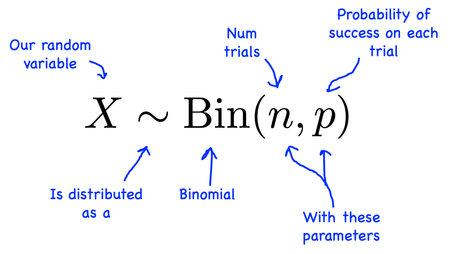
| Notation: | $X \sim \Bin(n, p)$ |
|---|---|
| Description: | Number of "successes" in $n$ identical, independent experiments each with probability of success $p$. |
| Parameters: | $n \in \{0, 1, \dots\}$, the number of experiments. $p \in [0, 1]$, the probability that a single experiment gives a "success". |
| Support: | $x \in \{0, 1, \dots, n\}$ |
| PMF equation: | $$\p(X=x) = {n \choose x}p^x(1-p)^{n-x}$$ |
| Expectation: | $\E[X] = n \cdot p$ |
| Variance: | $\var(X) = n \cdot p \cdot (1-p)$ |
| PMF graph: |
One way to think of the binomial is as the sum of $n$ Bernoulli variables. Say that $Y_i \sim \Ber(p)$ is an indicator Bernoulli random variable which is 1 if experiment $i$ is a success. Then if $X$ is the total number of successes in $n$ experiments, $X \sim \Bin(n, p)$: $$ X = \sum_{i=1}^n Y_i $$
Recall that the outcome of $Y_i$ will be 1 or 0, so one way to think of $X$ is as the sum of those 1s and 0s.
Binomial PMF
The most important property to know about a binomial is its PMF function:
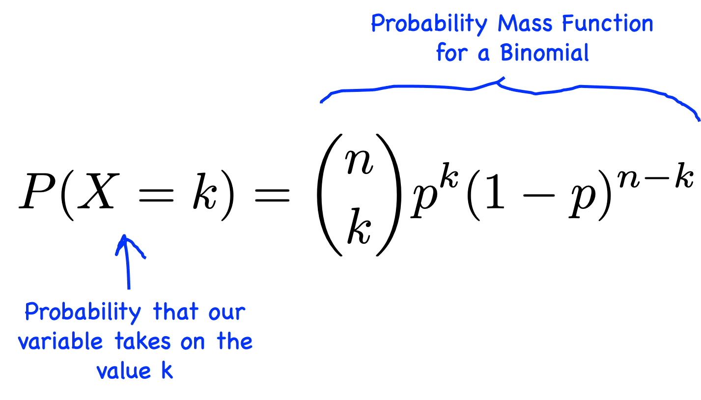
Recall, we derived this formula in Part 1. There is a complete example on the probability of $k$ heads in $n$ coin flips, where each flip is heads with probability $0.5$: Many Coin Flips. To briefly review, if you think of each experiment as being distinct, then there are ${n \choose k}$ ways of permuting $k$ successes from $n$ experiments. For any of the mutually exclusive permutations, the probability of that permutation is $p^k \cdot (1-p)^{n-k}$.
The name binomial comes from the term ${n \choose k}$ which is formally called the binomial coefficient.
Expectation of Binomial
There is an easy way to calculate the expectation of a binomial and a hard way. The easy way is to leverage the fact that a binomial is the sum of Bernoulli indicator random variables. $X = \sum_{i=1}^{n} Y_i$ where $Y_1$ is an indicator of whether the $i$th experiment was a success: $Y_i \sim \Ber(p)$. Since the expectation of the sum of random variables is the sum of expectations, we can add the expectation, $\E[Y_i] = p$, of each of the Bernoulli's: $$ \begin{align} \E[X] &= \E\Big[\sum_{i=1}^{n} Y_i\Big] && \text{Since }X = \sum_{i=1}^{n} Y_i \\ &= \sum_{i=1}^{n}\E[ Y_i] && \text{Expectation of sum} \\ &= \sum_{i=1}^{n}p && \text{Expectation of Bernoulli} \\ &= n \cdot p && \text{Sum $n$ times} \end{align} $$ The hard way is to use the definition of expectation: $$ \begin{align} \E[X] &= \sum_{i=0}^n i \cdot \p(X = i) && \text{Def of expectation} \\ &= \sum_{i=0}^n i \cdot {n \choose i} p^i(1-p)^{n-i} && \text{Sub in PMF} \\ & \cdots && \text{Many steps later} \\ &= n \cdot p \end{align} $$
Binomial Distribution in Python
As you might expect, you can use binomial distributions in code. The standardized library for binomials is scipy.stats.binom.
One of the most helpful methods that this package provides is a way to calculate the PMF. For example, say $X \sim \text{Bin}(n=5,p=0.6)$ and you want to find $\P(X=2)$ you could use the following code:
from scipy import stats

# define variables for x, n, and p
n = 5
p = 0.6
x = 2

# use scipy to compute the pmf
p_x = stats.binom.pmf(x, n, p)

# use the probability for future work
print(f'P(X = {x}) = {p_x}')
P(X = 2) = 0.2304Another particularly helpful function is the ability to generate a random sample from a binomial. For example, say $X \sim \Bin(n=10, p = 0.3)$ represents the number of requests to a website. We can draw 100 samples from this distribution using the following code:
from scipy import stats

# define variables for x, n, and p
n = 10
p = 0.3
x = 2

# use scipy to compute the pmf
samples = stats.binom.rvs(n, p, size=100)

# use the probability for future work
print(samples)
[4 5 3 1 4 5 3 1 4 6 5 6 1 2 1 1 2 3 2 5 2 2 2 4 4 2 2 3 6 3 1 1 4 2 6 2 4
 2 3 3 4 2 4 2 4 5 0 1 4 3 4 3 3 1 3 1 1 2 2 2 2 3 5 3 3 3 2 1 3 2 1 2 3 3
 4 5 1 3 7 1 4 1 3 3 4 4 1 2 4 4 0 2 4 3 2 3 3 1 1 4]
You might be wondering what a random sample is! A random sample is a randomly chosen assignment for our random variable. Above we have 100 such assignments. The probability that value $x$ is chosen is given by the PMF: $\p(X=x)$. You will notice that even though 8 is a possible assignment to the binomial above, in 100 samples we never saw the value 8. Why? Because $P(X=8) \approx 0.0014$. You would need to draw 1,000 samples before you would expect to see an 8.
There are also functions for getting the mean, the variance, and more. You can read the scipy.stats.binom documentation, especially the list of methods.