Binomial Approximation

There are times when it is exceptionally hard to numerically calculate probabilities for a binomial distribution, especially when $n$ is large. For example, say $X \sim \text{Bin}(n = 10000, p = 0.5)$ and you want to calculate $\p(X > 5500)$. The correct formula is: \begin{align} \p(X > 55) &= \sum_{i = 5500}^{10000} \p(X=x) \\ &= \sum_{i = 5500}^{10000}{10000 \choose i}p^i(1-p)^{10000-i} \end{align}

That is a difficult value to calculate. Luckily there is an easier way. For deep reasons which we will cover in our section on "uncertainty theory" it turns out that a binomial distribution can be very well approximated by both Normal distributions and Poisson distributions if $n$ is large enough.

Use the Poisson approximation when $n$ is large (>20) and $p$ is small (<0.05). A slight dependence between results of each experiment is ok

Use the Normal approximation when $n$ is large (>20), and $p$ is mid-ranged. Specifically it's considered an accurate approximation when the variance is greater then 10, in other words: $np(1-p)>10$. There are situations where either a Poisson or a Normal can be used to approximate a Binomial. In that situation go with the Normal!

Poisson Approximation

When defining the Poisson we proved that a Binomial in the limit as $n \rightarrow \infty$ and $p = \lambda/n$ is a Poisson. That same logic can be used to show that a Poisson is a great approximation for a Binomial when the Binomial has extreme values of $n$ and $p$. A Poisson random variable approximates Binomial where $n$ is large, $p$ is small, and $\lambda = np$ is “moderate”. Interestingly, to calculate the things we care about (PMF, expectation, variance) we no longer need to know $n$ and $p$. We only need to provide $\lambda$ which we call the rate. When approximating a Poisson with a Binomial, always choose $\lambda = n \cdot p$.

There are different interpretations of "moderate". The accepted ranges are $n > 20$ and $p < 0.05$ or $n > 100$ and $p < 0.1$.

Normal Approximation

For a Binomial where $n$ is large and $p$ is mid-ranged, a Normal can be used to approximate the Binomial. Let's take a side by side view of a normal and a binomial:

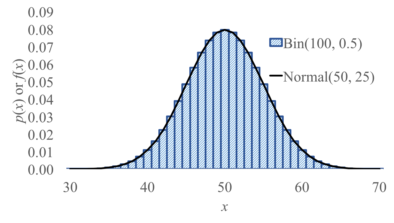
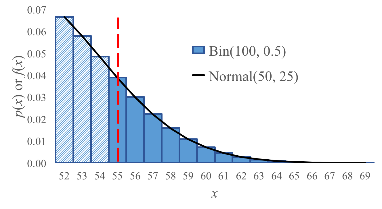
Lets say our binomial is a random variable $X \sim \text{Bin}(100, 0.5)$ and we want to calculate $P(X \geq 55)$. We could cheat by using the closest fit normal (in this case $Y \sim N(50, 25)$). How did we choose that particular Normal? Simply select one with a mean and variance that matches the Binomial expectation and variance. The binomial expectation is $np = 100 \cdot 0.5 = 50$. The Binomial variance is $np(1-p) = 100 \cdot 0.5 \cdot 0.5 = 25$.

You can use a Normal distribution to approximate a Binomial $X\sim \Bin(n,p)$. To do so define a normal $Y \sim (E[X], Var(X))$. Using the Binomial formulas for expectation and variance, $Y \sim (np, np(1-p))$. This approximation holds for large $n$ and moderate $p$. That gets you very close. However since a Normal is continuous and Binomial is discrete we have to use a continuity correction to discretize the Normal.