Continuous Distribution

So far, all random variables we have seen have been discrete. In all the cases we have seen in CS109 this meant that our RVs could only take on integer values. Now it's time for continuous random variables which can take on values in the real number domain ($\R$). Continuous random variables can be used to represent measurements with arbitrary precision (eg height, weight, time).

From Discrete to Continuous

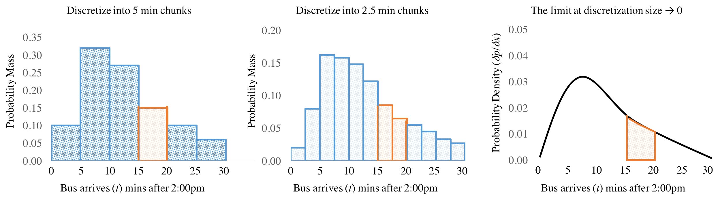
To make our transition from thinking about discrete random variables, to thinking about continuous random variables, lets start with a thought experiment: Imagine you are running to catch the bus. You know that you will arrive at 2:15pm but you don't know exactly when the bus will arrive, and want to think of the arrival time in minutes past 2pm as a random variable $T$ so that you can calculate the probability that you will have to wait more than five minutes $P(15 < T < 20)$.

We immediately face a problem. For discrete distributions we would describe the probability that a random variable takes on exact values. This doesn't make sense for continuous values, like the time the bus arrives. As an example, what is the probability that the bus arrives at exactly 2:17pm and 12.12333911102389234 seconds? Similarly, if I were to ask you: what is the probability of a child being born with weight exactly equal to 3.523112342234 kilos, you might recognize that question as ridiculous. No child will have precisely that weight. Real values can have infinite precision and as such it is a bit mind boggling to think about the probability that a random variable takes on a specific value.

Instead, let's start by discretizing time, our continuous variable, by breaking it into 5 minute chunks. We can now think about something like, the probability that the bus arrives between 2:00p and 2:05 as an event with some probability (see figure below on the left). Five minute chunks seem a bit coarse. You could imagine that instead, we could have discretized time into 2.5 minute chunks (figure in the center). In this case the probability that the bus shows up between 15 mins and 20 mins after 2pm is the sum of two chunks, shown in orange. Why stop there? In the limit we could keep breaking time down into smaller and smaller pieces. Eventually we will be left with a derivative of probability at each moment of time, where the probability that $P(15 < T < 20)$ is the integral of that derivative between 15 and 20 (figure on the right).

Probability Density Functions

In the world of discrete random variables, the most important property of a random variable was its probability mass function (PMF) that would tell you the probability of the random variable taking on any value. When we move to the world of continuous random variables, we are going to need to rethink this basic concept. In the continuous world, every random variable instead has a Probability Density Function (PDF) which defines the relative likelihood that a random variable takes on a particular value. We traditionally use the symbol $f$ for the probability density function and write it in one of two ways: $$ f(X=x) \quad \or \quad f(x) $$ Where the notation on the right hand side is shorthand and the lowercase $x$ implies that we are talking about the relative likelihood of a continuous random variable which is the upper case $X$. Like in the bus example, the PDF is the derivative of probability at all points of the random variable. This means that the PDF has the important property that you can integrate over it to find the probability that the random variable takes on values within a range $(a, b)$.

Definition: Continuous Random Variable

$X$ is a Continuous Random Variable if there is a Probability Density Function (PDF) $f(x)$ that takes in real valued numbers $x$ such that: $$ \begin{align*} &\P(a \leq X \leq b) = \int_a^b f(x) \d x \end{align*} $$ The following properties must also hold. These preserve the axiom that $P(a \leq X \leq b)$ is a probability: $$ \begin{align*} &0 \leq \P(a \leq X \leq b) \leq 1 \\ &\P(-\infty < X < \infty) = 1 \end{align*} $$

A common misconception is to think of $f(x)$ as a probability. It is instead what we call a probability density. It represents probability/unit of $X$. Generally this is only meaningful when we either take an integral over the PDF or we compare probability densities. As we mentioned when motivating probability densities, the probability that a continuous random variable takes on a specific value (to infinite precision) is 0.

$$ \P(X = a) = \int_a^a f(x) \d x = 0 $$

That is pretty different than in the discrete world where we often talked about the probability of a random variable taking on a particular value.

Cumulative Distribution Function

Having a probability density is great, but it means we are going to have to solve an integral every single time we want to calculate a probability. To avoid this unfortunate fate, we are going to use a standard called a cumulative distribution function (CDF). The CDF is a function which takes in a number and returns the probability that a random variable takes on a value less than that number. It has the pleasant property that, if we have a CDF for a random variable, we don't need to integrate to answer probability questions!

For a continuous random variable $X$ the Cumulative Distribution Function, written $F(x)$ is: $$ \begin{align*} &F(x) = P(X \leq x) = \int_{-\infty}^{x} f(x)\d x \end{align*} $$

Why is the CDF the probability that a random variable takes on a value less than the input value as opposed to greater than? It is a matter of convention. But it is a useful convention. Most probability questions can be solved simply by knowing the CDF (and taking advantage of the fact that the integral over the range $-\infty$ to $\infty$ is 1. Here are a few examples of how you can answer probability questions by just using a CDF: \begin{align*} &\text{Probability Query} && \text{Solution} && \text{Explanation} \\ &\P(X < a) && F(a) && \text{That is the definition of the CDF}\\ &\P(X \leq a) && F(a) && \text{Trick question. }\P(X = a) = 0\\ &\P(X > a) && 1 - F(a) && \P(X < a) + \P(X > a) = 1 \\ &\P(a < X < b) && F(b) - F(a) && F(a) + \P(a < X < b) = F(b)\\ \end{align*}

The continuous distribution also exists for discrete random variables, but there is less utility to a CDF in the discrete world as none of our discrete random variables had "closed form" (eg without any summation) functions for the CDF: \begin{align*} F_X(a) = \sum_{i = 1}^a P(X = i) \end{align*}

Solving for Constants

Let $X$ be a continuous random variable with PDF: \begin{align*} f(x) = \begin{cases} C(4x - 2x^2) &\text{when } 0 < x < 2 \\ 0 & \text{otherwise} \end{cases} \end{align*} In this function, $C$ is a constant. What value is $C$? Since we know that the PDF must sum to 1: \begin{align*} &\int_0^2 C(4x - 2x^2) \d x = 1 \\ &C\left(2x^2 - \frac{2x^3}{3}\right)\bigg|_0^2 = 1 \\ &C\left(\left(8 - \frac{16}{3}\right) - 0 \right) = 1 \\ &C = 3/8 \end{align*} Now that we know $C$, what is $\P(X > 1)$? \begin{align*} \P(X > 1) &=\int_1^{\infty}f(x) \d x \\ &= \int_1^2 \frac{3}{8}(4x - 2x^2) \d x \\ &= \frac{3}{8}\left(2x^2 - \frac{2x^3}{3}\right)\bigg|_1^2 \\ &= \frac{3}{8}\left[\left(8 - \frac{16}{3}\right) - \left(2 - \frac{2}{3}\right)\right] = \frac{1}{2} \end{align*}

Expectation and Variance of Continuous Variables

For continuous RV $X$: \begin{align*} &E[X] = \int_{-\infty}^{\infty} x f(x) dx \\ &E[g(X)] = \int_{-\infty}^{\infty} g(x) f(x) dx \\ &E[X^n] = \int_{-\infty}^{\infty} x^n f(x) dx \end{align*}

For both continuous and discrete RVs: \begin{align*} &E[aX + b] = aE[X] + b\\ &\text{Var}(X) = E[(X - \mu)^2] = E[X^2] - (E[X])^2 \\ &\text{Var}(aX + b) = a^2 \text{Var}(X) \end{align*}