Variance
Definition: Variance of a Random Variable
The variance is a measure of the "spread" of a random variable around the mean. Variance for a random variable, X, with expected value $\E[X] = µ$ is: $$ \var(X) = \E[(X–µ)^2] $$ Semantically, this is the average distance of a sample from the distribution to the mean. When computing the variance often we use a different (equivalent) form of the variance equation: $$ \begin{align} \var(X) &= \E[X^2] - \E[X]^2 \end{align} $$
In the last section we showed that Expectation was a useful summary of a random variable (it calculates the "weighted average" of the random variable). One of the next most important properties of random variables to understand is variance: the measure of spread.
To start, let's consider probability mass functions for three sets of graders. When each of them grades an assigment, meant to receive a 70/100, they each have a probability distribution of grades that they could give.
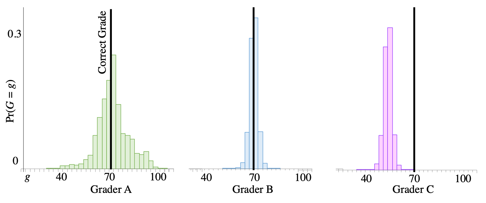 Distributions of three types of peer graders. Data is from a massive online course.
The distribution for graders in group $C$ has a different expectation. The average grade that they give when grading an assignment worth 70 is a 55/100. That is clearly not great! But what is the difference between graders $A$ and $B$? Both of them have the same expected value (which is equal to the correct grade). The graders in group $A$ have a higher "spread". When grading an assignment worth 70, they have a reasonable chance of giving it a 100, or of giving it a 40. Graders in group $B$ have much less spread. Most of the probability mass is close to 70. You want graders like those in group $B$: in expectation they give the correct grade, and they have low spread. As an aside: scores in group $B$ came from a probabilistic algorithm over peer grades.
Theorists wanted a number to describe spread. They invented variance to be the average of the distance between values that the random variable could take on and the mean of the random variable. There are many reasonable choices for the distance function, probability theorists chose squared deviation from the mean: $$ \var(X) = \E[(X–µ)^2] $$
Proof: $\var(X) = \E[X^2] - \E[X]^2$
It is much easier to compute variance using $\E[X^2] - \E[X]^2$. You certainly don't need to know why its an equivalent expression, but in case you were wondering, here is the proof.
$$ \begin{align} \var(X) &= \E[(X–µ)^2] && \text{Note: } \mu = \E[X]\\ &= \sum_x(x-\mu)^2 \p(x) && \text{Definition of Expectation}\\ &= \sum_x (x^2 -2\mu x + \mu^2) \P(x) && \text{Expanding the square}\\ &= \sum_x x^2\P(x)- 2\mu \sum_x x \P(x) + \mu^2 \sum_x \P(x) && \text{Propagating the sum}\\ &= \sum_x x^2\P(x)- 2\mu \E[X] + \mu^2 \sum_x \P(x) && \text{Substitute def of expectation}\\ &= \E[X^2]- 2\mu \E[X] + \mu^2 \sum_x \P(x) && \text{LOTUS } g(x) = x^2 \\ &= \E[X^2]- 2\mu \E[X] + \mu^2 && \text{Since }\sum_x \P(x) = 1\\ &= \E[X^2]- 2\E[X]^2 + \E[X]^2 && \text{Since }\mu = \E[X]\\ &= \E[X^2]- \E[X]^2 && \text{Cancelation}\\ \end{align} $$Standard Deviation
Variance is especially useful for comparing the "spread" of two distributions and it has the useful property that it is easy to calculate. In general a larger variance means that there is more deviation around the mean — more spread. However, if you look at the leading example, the units of variance are the square of points. This makes it hard to interpret the numerical value. What does it mean that the spread is 52 points$^2$? A more interpretable measure of spread is the square root of Variance, which we call the Standard Deviation $\std(X) = \sqrt{\var(X)}$. The standard deviation of our grader is 7.2 points. In this example folks find it easier to think of spread in points rather than points$^2$. As an aside, the standard deviation is the average distance of a sample (from the distribution) to the mean, using the euclidean distance function.
Variance with Continuous Random Variables
Later in the course reader we will learn about continuous random variables. Variance for those types of random variables is very similar. See Continuos Random Variables for details.