Continuous Joint
Random variables $X$ and $Y$ are Jointly Continuous if there exists a joint Probability Density Function (PDF) $f$ such that: \begin{align*} P(a_1 < X \leq a_2,b_1 < Y \leq b_2) = \int_{a_1}^{a_2} \int_{b_1}^{b_2} f(X=x,Y=y)\d y \text{ } \d x \end{align*}
Using the PDF we can compute marginal probability densities: \begin{align*} f(X=a) &= \int_{-\infty}^{\infty}f(X=a,Y=y)\d y \\ f(Y=b) &= \int_{-\infty}^{\infty}f(X=x,Y=b)\d x \end{align*}
Let $F(x,y)$ be the Cumulative Density Function (CDF): \begin{align*} P(a_1 < X \leq a_2,b_1 < Y \leq b_2) = F(a_2,b_2) - F(a_1,b_2) + F(a_1,b_1) - F(a_2,b_1) \end{align*}
From Discrete Joint to Continuous Joint
Thinking about multiple continuous random variables jointly can be unintuitive at first blush. But we can turn to our helpful trick that we can use to understand continuous random variables: start with a discrete approximation. Consider the example of creating the CS109 seal. It was generated by throwing half a million darts at an image of the stanford logo (keeping all the pixels that get hit by at least one dart). The darts could hit any continuous location on the logo, and, the locations are not equally likely. Instead, the location a dart hits is goverened by a joint continuous distribution. In this case there are only two simultaneous random variables, the x location of the dart and the y location of the dart. Each random variable is continuous (it takes on real numbers). Thinking about the joint probability density function is easier by first considering a discretization. I am going to break the dart landing area into 25 discrete buckets:
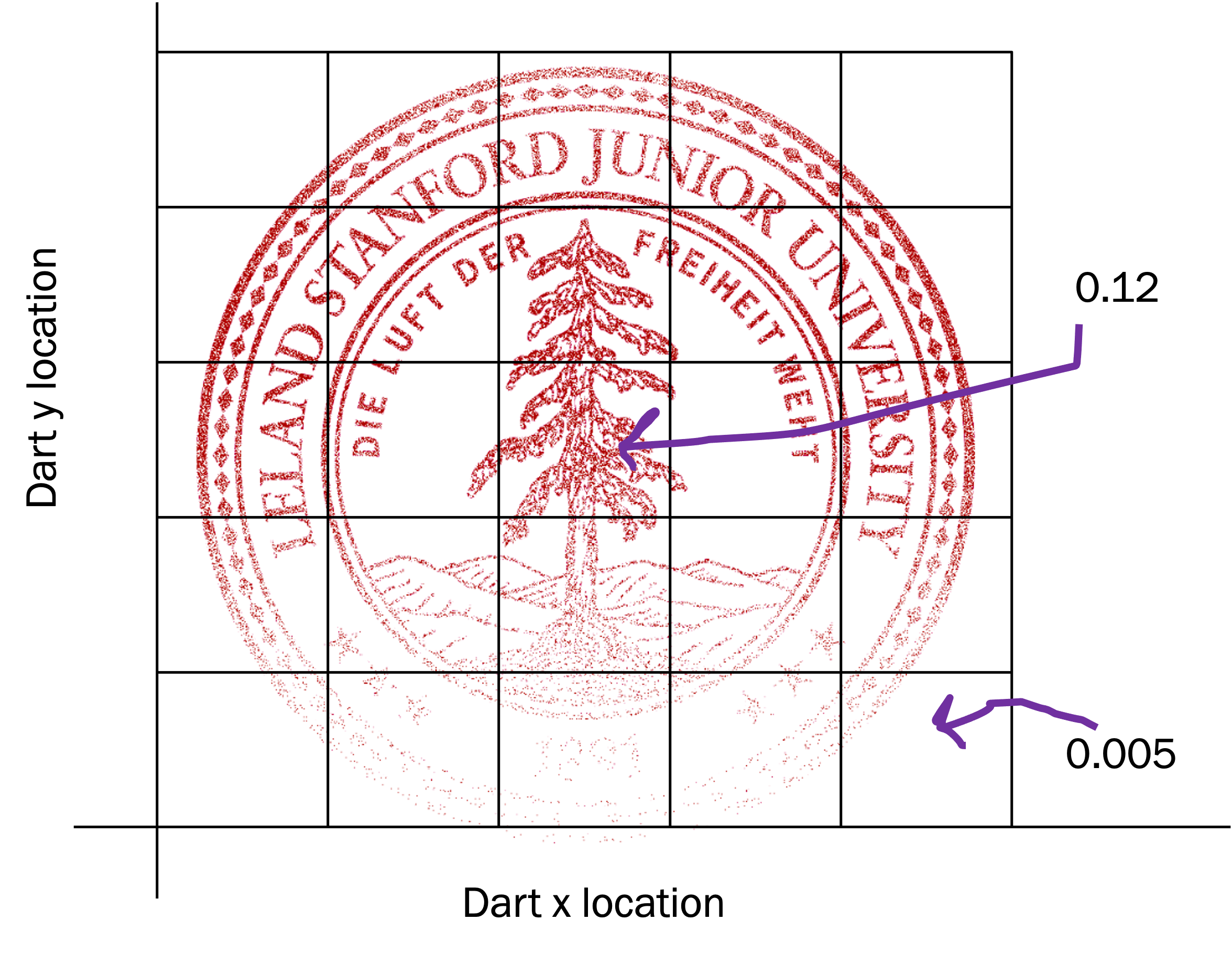
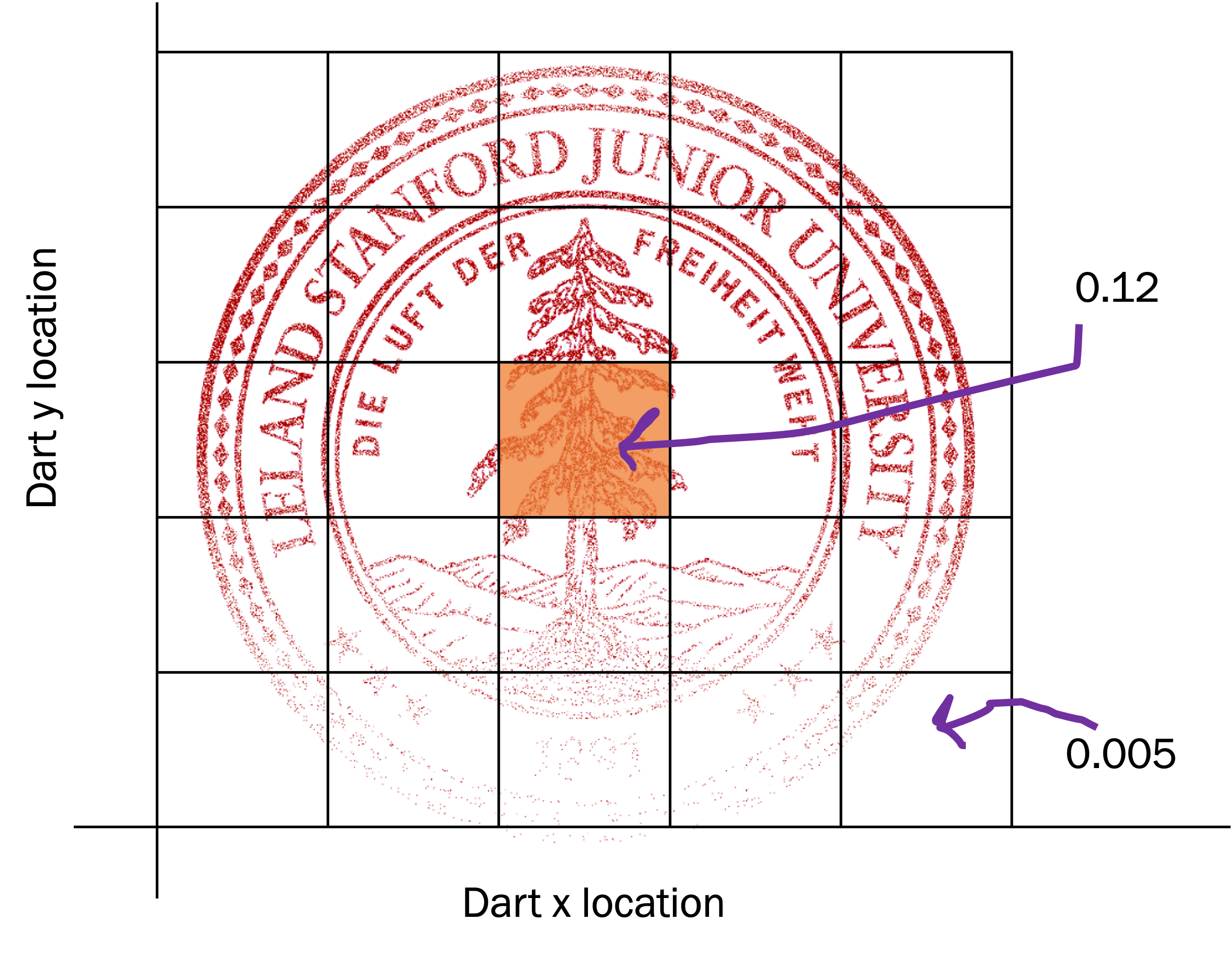
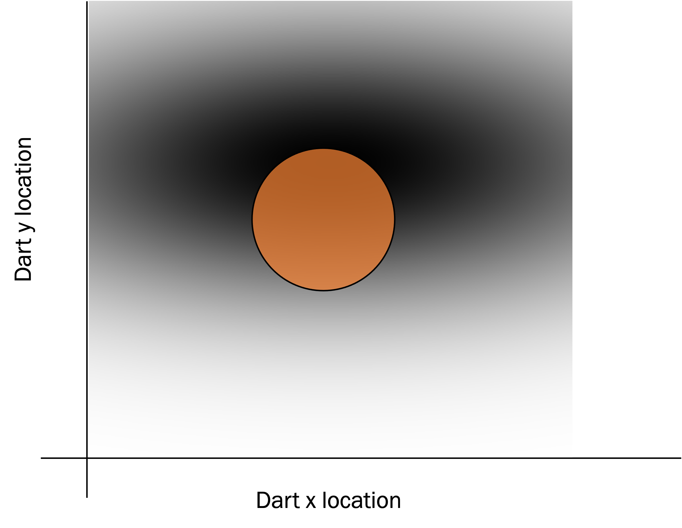
On the left is a visualization of the probability mass of this joint distribution, and on the right is a visualization of how we could answer the question: what is the probability that a dart hits within a certain distance of the center. For each bucket there is a single number, the probability that a dart will fall into that particular bucket (these probabilities are mutually exclusive and sum to 1).
Of course this discretization only approximates the joint probability distribution. In order to get a better approximation we could create more fine-grained discretizations. In the limit we can make our buckets infinitely small, and the value associated with each bucket becomes a second derivative of probability.

To represent the 2D probability density in a graph, we use the darkness of a value to represent the density (darker means more density). Another way to visualize this distribution is from an angle. This makes it easier to realize that this is a function with two inputs and one output. Below is an different visualization of the exact same density function:
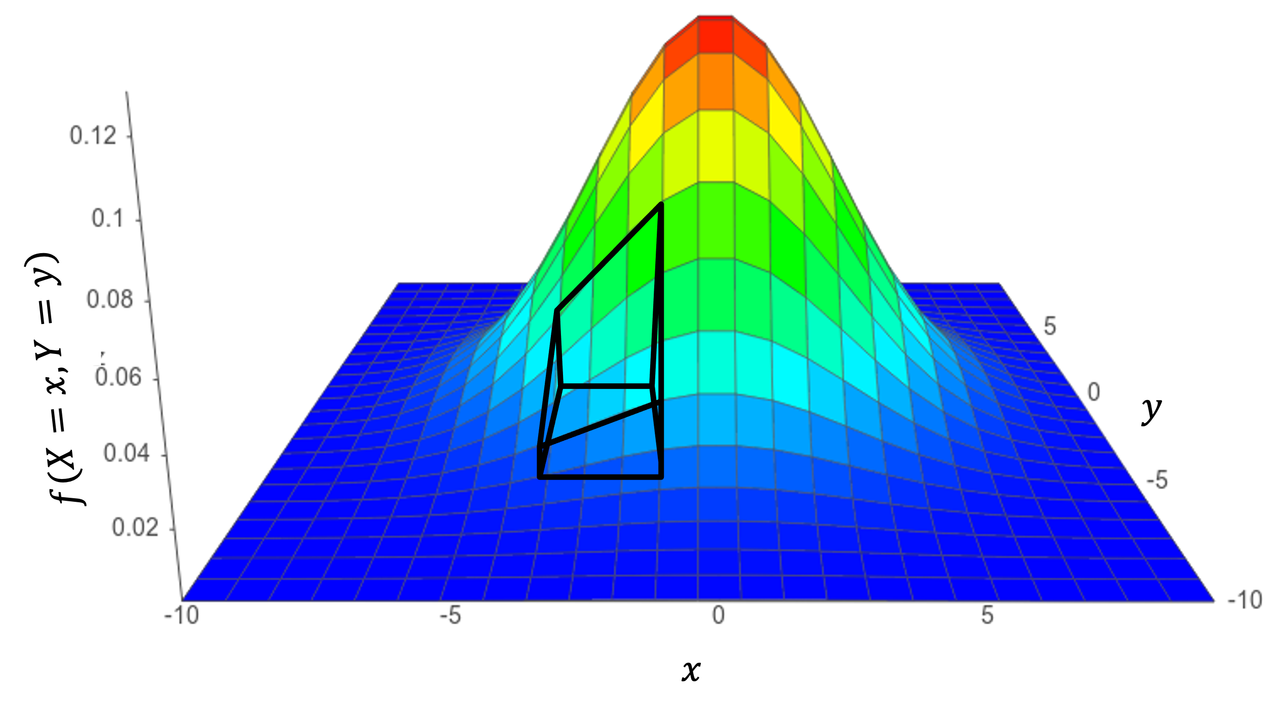
Just like in the single random variable case, we are now representing our belief in the continuous random variables as densities rather than probabilities. Recall that a density represents a relative belief. If the density of $f(X = 1.1, Y = 0.9)$ is twice as high as the density that $f(X = 1.1, Y = 1.1)$ the function is expressing that it is twice as likely to find the particular combination of $X = 1.1$ and $Y=0.9$.
Multivariate Gaussian
The density that is depicted in this example happens to be a particular of joint continuous distribution called Multivariate Gaussian. In fact it is a special case where all of the constituent variables are independent.
Example: Gaussian Blur
In the same way that many single random variables are assumed to be gaussian, many joint random variables may be assumed to be Multivariate Gaussian. Consider this example of Gaussian Blur:
In image processing, a Gaussian blur is the result of blurring an image by a Gaussian function. It is a widely used effect in graphics software, typically to reduce image noise. A Gaussian blur works by convolving an image with a 2D independent multivariate gaussian (with means of 0 and equal valued standard deviations).

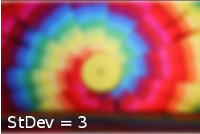
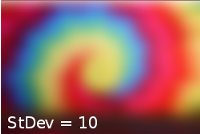
In order to use a Gaussian blur, you need to be able to compute the probability mass of that 2D gaussian in the space of pixels. Each pixel is given a weight equal to the probability that X and Y are both within the pixel bounds. The center pixel covers the area where $-0.5 ≤ x ≤ 0.5$ and $-0.5 ≤ y ≤ 0.5$. Let's do one step in computing the Gaussian function discretized over image space. What is the weight of the center pixel for gaussian blur with a multivariate gaussian which has means of 0 and standard deviation of 3?
Let $\vec{B}$ be the multivariate gaussian, $\vec{B} \sim \N(\vec{\mu} = [0,0], \vec{\sigma} = [3,3])$. Let's compute the CDF of this multivariate gaussian $F(x_1,x_2)$: \begin{align*} F(x_1,x_2) &= \prod_{i=1}^n \Phi(\frac{x_i-\mu_i}{\sigma_i}) \\ &= \Phi(\frac{x_1-\mu_1}{\sigma_1}) \cdot \Phi(\frac{x_2-\mu_2}{\sigma_2}) \\ &= \Phi(\frac{x_1}{3}) \cdot \Phi(\frac{x_2}{3}) \end{align*}
Now we are ready to calculate the weight of the center pixel: \begin{align*} \P&(-0.5 < X_1 \leq 0.5,-0.5 < X_2 \leq 0.5) \\ &= F(0.5,0.5) - F(-0.5,0.5) + F(-0.5,-0.5) - F(0.5,-0.5) \\ &=\Phi(\frac{0.5}{3}) \cdot \Phi(\frac{0.5}{3}) - \Phi(\frac{-0.5}{3}) \cdot \Phi(\frac{0.5}{3}) + \Phi(\frac{-0.5}{3}) \cdot \Phi(\frac{-0.5}{3}) - \Phi(\frac{0.5}{3}) \cdot \Phi(\frac{-0.5}{3})\\ &\approx 0.026 \end{align*}
How can this 2D gaussian blur the image? Wikipedia explains: "Since the Fourier transform of a Gaussian is another Gaussian, applying a Gaussian blur has the effect of reducing the image's high-frequency components; a Gaussian blur is a low pass filter" [2].