Inference

So far we have set the foundation for how we can represent probabilistic models with multiple random variables. These models are especially useful because they let us perform a task called "inference" where we update our belief about one random variable in the model, conditioned on new information about another. Inference in general is hard! In fact, it has been proven that in the worst case, the inference task, can be NP-Hard where $n$ is the number of random variables [1].

First we are going to practice it with two random variables (in this section). Then, later in this unit we are going to talk about inference in the general case, with many random variables.

Earlier we looked at conditional probabilities for events. The first task in inference is to understand how to combine conditional probabilities and random variables. The equations for both the discrete and continuous case are intuitive extensions of our understanding of conditional probability:

The Discrete Conditional

The discrete case, where every random variable in your model is discrete, is a straightforward combination of what you know about conditional probability (which you learned in the context of events). Recall that every relational operator applied to a random variable defines an event. As such the rules for conditional probability directly apply: The conditional probability mass function (PMF) for the discrete case:

In the presence of multiple random variables, it becomes increasingly useful to use shorthand! The above definition is identical to this notation where a lowercase symbol such as $x$ is short hand for the event $X=x$: \begin{align*} \P(x|y)=\frac{P(x,y)}{P(y)} \end{align*} The conditional definition works for any event and as such we can also write conditionals using cumulative density functions (CDFs) for the discrete case: \begin{align*} \P(X \leq a | Y=y) &= \frac{\P(X \leq a, Y=y)}{\p(Y=y)} \\ &= \frac{\sum_{x\leq a} \P(X=x,Y=y)}{\P(Y=y)} \end{align*} Here is a neat result: this last term can be rewritten, by a clever manipulation. We can make the sum extend over the whole fraction: \begin{align*} \P(X \leq a | Y=y) &= \frac{\sum_{x\leq a} \P(X=x,Y=y)}{\P(Y=y)} \\ &= \sum_{x\leq a} \frac{\P(X=x,Y=y)}{\P(Y=y)} \\ &= \sum_{x\leq a} \P(X=x|Y=y) \end{align*}

In fact it becomes straight forward to translate the rules of probability (such as Bayes' Theorem, law of total probability, etc) to the language of discrete random variables: we simply need to recall that every relational operator applied to a random variable defines an event.

Mixing Discrete and Continuous

What happens when we want to reason about continuous random variables using our rules of probability (such as Bayes' Theorem, law of total probability, chain rule, etc)? There is a simple practical answer: the rules still apply, but we have to replace probability terminology with probability density functions. As a concrete example let's look at Bayes' Theorem with one continuous random variable.

These equations might seem complicated since they mix probability densities and probabilities. Why should we believe that they are correct? First, observe that anytime the random variable on the left hand side of the conditional is continuous, we use a density, whenever it is discrete, we use a probability. This result can be derived by making the observation: $$ \P(X = x) = f(X=x) \cdot \epsilon_x $$

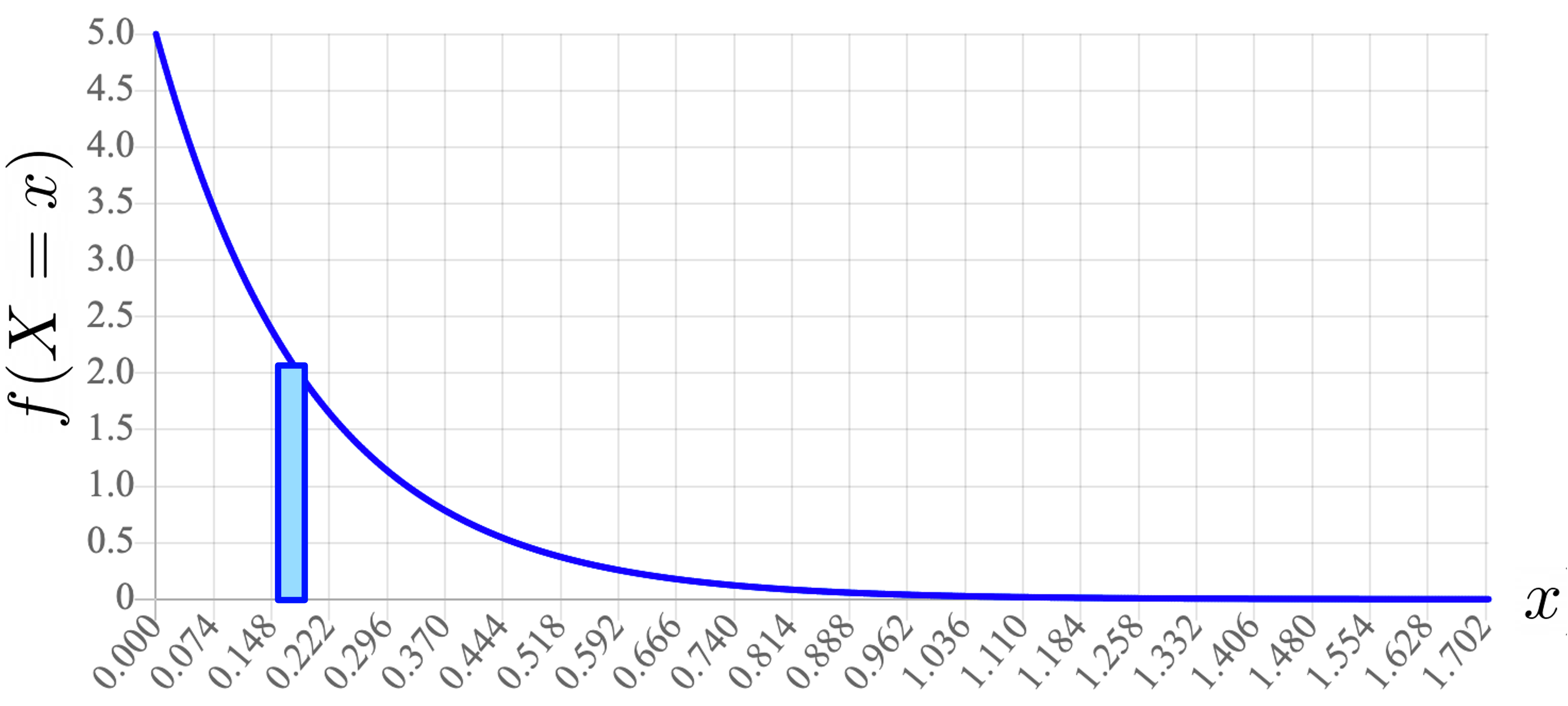
In the limit as $\epsilon_x \rightarrow 0$. In order to obtain a probability from a density function is to integrate under the function. If you wanted to approximate the probability that $X = x$ you could consider the area created by a rectangle which has height $f(X=x)$ and some very small width. As that width gets smaller, your answer becomes more accurate:

A value of $\epsilon_x$ is problematic if it is left in a formula. However, if we can get them to cancel, we can arrive at a working equation. This is the key insight used to derive the rules of probability in the context of one or more continuous random variables. Again, let $X$ be continuous random variable and let $N$ be a discrete random variable: \begin{align*} \p(N=n|X=x) &= \frac{P(X=x|N=n)\p(N=n)}{P(X=x)} &&\text{Bayes' Theorem}\\ &= \frac{f(X=x|N=n) \cdot \epsilon_x \cdot \p(N=n)}{f(X=x) \cdot \epsilon_x} &&\P(X = x) = f(X=x) \cdot \epsilon_x \\ &= \frac{f(X=x|N=n) \cdot \p(N=n)}{f(X=x)} &&\text{Cancel } \epsilon_x \\ \end{align*}

This strategy applies beyond Bayes' Theorem. For example here is a version of the Law of Total Probability when $X$ is continuous and $N$ is discrete: \begin{align*} f(X=x) &= \sum_{n \in N} f(X=x | N = n) \p(N = n) \end{align*}

Probability Rules with Continuous Random Variables

The strategy used in the above section can be used to derive the rules of probability in the presence of continuous random variables. The strategy also works when there are multiple continuous random variables. For example here is Bayes' Theorem with two continuous random variables.

Example: Inference with a Continuous Variable

Consider the following question: