Sampling
In this section we are going to talk about statistics calculated on samples from a population. We are then going to talk about probability claims that we can make with respect to the original population -- a central requirement for most scientific disciplines.
Let's say you are the king of Bhutan and you want to know the average happiness of the people in your country. You can't ask every single person, but you could ask a random subsample. In this next section we will consider principled claims that you can make based on a subsample. Assume we randomly sample 200 Bhutanese and ask them about their happiness. Our data looks like this: ${72, 85, \dots, 71}$. You can also think of it as a collection of $n$ = 200 I.I.D. (independent, identically distributed) random variables ${X_1, X_2, \dots, X_n}$.
Understanding Samples
The idea behind sampling is simple, but the details and the mathematical notation can be complicated. Here is a picture to show you all of the ideas involved:
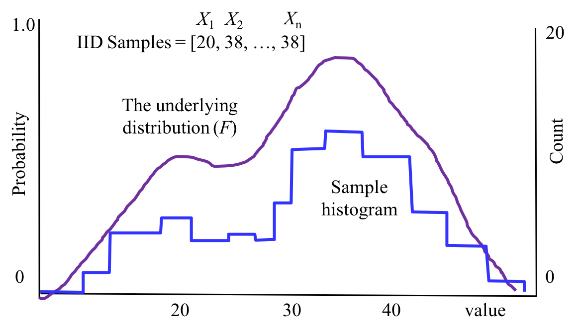
The theory is that there is some large population (for example the 774,000 people who live in Bhutan). We collect a sample of $n$ people at random, where each person in the population is equally likely to be in our sample. From each person we record one number (for example their reported happiness). We are going to call the number from the ith person we sampled $X_i$. One way to visualize your samples ${X_1, X_2, \dots, X_n}$ is to make a histogram of their values.
We make the assumption that all of our $X_i$s are identically distributed. That means that we are assuming there is a single underlying distribution $F$ that we drew our samples from. Recall that a distribution for discrete random variables should define a probability mass function.
Estimating Mean and Variance from Samples
We assume that the data we look at are IID from the same underlying distribution ($F$) with a true mean ($\mu$) and a true variance ($\sigma^2$). Since we can't talk to everyone in Bhutan we have to rely on our sample to estimate the mean and variance. From our sample we can calculate a sample mean ($\bar{X}$) and a sample variance ($S^2$). These are the best guesses that we can make about the true mean and true variance. \begin{align*} \bar{X} &= \sum_{i=1}^n \frac{X_i}{n} \\ S^2 &= \frac{1}{n-1}\sum_{i=1}^n (X_i - \bar{X})^2 \end{align*} The first question to ask is, are those unbiased estimates? Yes. Unbiased, means that if we were to repeat this sampling process many times, the expected value of our estimates should be equal to the true values we are trying to estimate. We will prove that that is the case for $\bar{X}$. The proof for $S^2$ is in lecture slides. \begin{align*} E[\bar{X}] &= E[\sum_{i=1}^n \frac{X_i}{n}] = \frac{1}{n}E\left[\sum_{i=1}^n X_i\right] \\ &= \frac{1}{n}\sum_{i=1}^n E[X_i] = \frac{1}{n}\sum_{i=1}^n \mu = \frac{1}{n}n\mu = \mu \end{align*}
The equation for sample mean seems related to our understanding of expectation. The same could be said about sample variance except for the surprising $(n-1)$ in the denominator of the equation. Why $(n-1)$? That denominator is necessary to make sure that the $E[S^2] = \sigma^2$.
The intuition behind the proof is that sample variance calculates the distance of each sample to the sample mean, not the true mean. The sample mean itself varies, and we can show that its variance is also related to the true variance.
Standard Error
Ok, you convinced me that our estimates for mean and variance are not biased. But now I want to know how much my sample mean might vary relative to the true mean. \begin{align*} \text{Var}(\bar{X}) &= \text{Var}(\sum_{i=1}^n \frac{X_i}{n}) = \left(\frac{1}{n}\right)^2 \text{Var}\left(\sum_{i=1}^n X_i\right) \\ &= \left(\frac{1}{n}\right)^2 \sum_{i=1}^n\text{Var}( X_i) =\left(\frac{1}{n}\right)^2 \sum_{i=1}^n \sigma^2 = \left(\frac{1}{n}\right)^2 n \sigma^2 = \frac{\sigma^2}{n}\\ &\approx \frac{S^2}{n} \\ \text{Std}(\bar{X}) &\approx \sqrt{\frac{S^2}{n}} \end{align*}
That term, Std($\bar{X}$), has a special name. It is called the standard error and its how you report uncertainty of estimates of means in scientific papers (and how you get error bars). Great! Now we can compute all these wonderful statistics for the Bhutanese people. But wait! You never told me how to calculate the Std($S^2$). That is hard because the central limit theorem doesn't apply to the computation of $S^2$. Instead we will need a more general technique. See the next chapter: Bootstrapping
Let's say we calculate the our sample of happiness has $n$ = 200 people. The sample mean is $\bar{X} = 83$ (what is the unit here? happiness score?) and the sample variance is $S^2 = 450$. We can now calculate the standard error of our estimate of the mean to be 1.5. When we report our results we will say that our estimate of the average happiness score in Bhutan is 83 $\pm$ 1.5. Our estimate of the variance of happiness is 450 $\pm$ ?.