Logistic Regression

Logistic Regression is a classification algorithm (I know, terrible name. Perhaps Logistic Classification would have been better) that works by trying to learn a function that approximates $\P(y|x)$. It makes the central assumption that $\P(y|x)$ can be approximated as a sigmoid function applied to a linear combination of input features. It is particularly important to learn because logistic regression is the basic building block of artificial neural networks.

Mathematically, for a single training datapoint ($\mathbf{x}, y)$ Logistic Regression assumes: \begin{align*} P(Y=1|\mathbf{X}=\mathbf{x}) &= \sigma(z) \text{ where } z = \theta_0 + \sum_{i=1}^m \theta_i x_i \end{align*} This assumption is often written in the equivalent forms: \begin{align*} P(Y=1|\mathbf{X}=\mathbf{x}) &=\sigma(\mathbf{\theta}^T\mathbf{x}) &&\text{ where we always set $x_0$ to be 1}\\ P(Y=0|\mathbf{X}=\mathbf{x}) &=1-\sigma(\mathbf{\theta}^T\mathbf{x}) &&\text{ by total law of probability} \end{align*} Using these equations for probability of $Y|X$ we can create an algorithm that selects values of theta that maximize that probability for all data. I am first going to state the log probability function and partial derivatives with respect to theta. Then later we will (a) show an algorithm that can chose optimal values of theta and (b) show how the equations were derived.

An important thing to realize is that: given the best values for the parameters ($\theta$), logistic regression often can do a great job of estimating the probability of different class labels. However, given bad , or even random, values of $\theta$ it does a poor job. The amount of ``intelligence" that you logistic regression machine learning algorithm has is dependent on having good values of $\theta$.

Notation

Before we get started I want to make sure that we are all on the same page with respect to notation. In logistic regression, $\theta$ is a vector of parameters of length $m$ and we are going to learn the values of those parameters based off of $n$ training examples. The number of parameters should be equal to the number of features of each datapoint.

Two pieces of notation that we use often in logistic regression that you may not be familiar with are: \begin{align*} \mathbf{\theta}^T\mathbf{x} &= \sum_{i=1}^m \theta_i x_i = \theta_1 x_1 + \theta_2 x_2 + \dots + \theta_m x_m && \text{dot product, aka weighted sum}\\ \sigma(z) &= \frac{1}{1+ e^{-z}} && \text{sigmoid function} \end{align*}

Log Likelihood

In order to chose values for the parameters of logistic regression we use Maximum Likelihood Estimation (MLE). As such we are going to have two steps: (1) write the log-likelihood function and (2) find the values of $\theta$ that maximize the log-likelihood function.

The labels that we are predicting are binary, and the output of our logistic regression function is supposed to be the probability that the label is one. This means that we can (and should) interpret the each label as a Bernoulli random variable: $Y \sim \text{Bern}(p)$ where $p = \sigma(\theta^T \textbf{x})$.

To start, here is a super slick way of writing the probability of one datapoint (recall this is the equation form of the probability mass function of a Bernoulli): \begin{align*} P(Y=y | X = \mathbf{x}) = \sigma({\mathbf{\theta}^T\mathbf{x}})^y \cdot \left[1 - \sigma({\mathbf{\theta}^T\mathbf{x}})\right]^{(1-y)} \end{align*}

Now that we know the probability mass function, we can write the likelihood of all the data: \begin{align*} L(\theta) =& \prod_{i=1}^n P(Y=y^{(i)} | X = \mathbf{x}^{(i)}) && \text{The likelihood of independent training labels}\\ =& \prod_{i=1}^n \sigma({\mathbf{\theta}^T\mathbf{x}^{(i)}})^{y^{(i)}} \cdot \left[1 - \sigma({\mathbf{\theta}^T\mathbf{x}^{(i)}})\right]^{(1-y^{(i)})} && \text{Substituting the likelihood of a Bernoulli} \end{align*} And if you take the log of this function, you get the reported Log Likelihood for Logistic Regression. The log likelihood equation is: \begin{align*} LL(\theta) = \sum_{i=1}^n y^{(i)} \log \sigma(\mathbf{\theta}^T\mathbf{x}^{(i)}) + (1-y^{(i)}) \log [1 - \sigma(\mathbf{\theta}^T\mathbf{x}^{(i)})] \end{align*}

Recall that in MLE the only remaining step is to chose parameters ($\theta$) that maximize log likelihood.

Gradient of Log Likelihood

Gradient Descent Optimization

Our goal is to choosing parameters ($\theta$) that maximize likelihood, and we know the partial derivative of log likelihood with respect to each parameter. We are ready for our optimization algorithm.

In the case of logistic regression we can't solve for $\theta$ mathematically. Instead we use a computer to chose $\theta$. To do so we employ an algorithm called gradient descent (a classic in optimization theory). The idea behind gradient descent is that if you continuously take small steps downhill (in the direction of your negative gradient), you will eventually make it to a local minima. In our case we want to maximize our likelihood. As you can imagine, minimizing a negative of our likelihood will be equivalent to maximizing our likelihood.

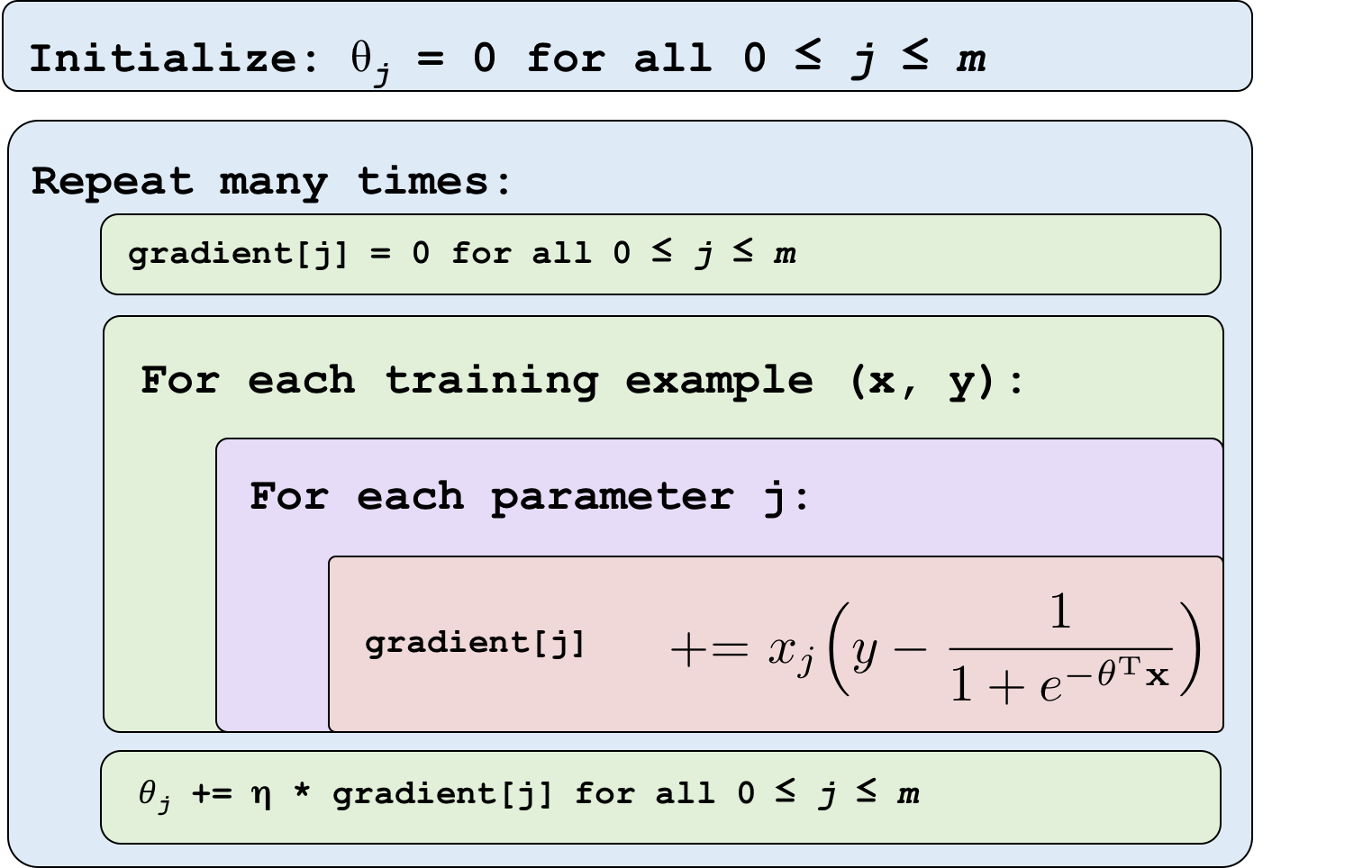
The update to our parameters that results in each small step can be calculated as: \begin{align*} \theta_j^{\text{ new}} &= \theta_j^{\text{ old}} + \eta \cdot \frac{\partial LL(\theta^{\text{ old}})}{\partial \theta_j^{\text{ old}}} \\ &= \theta_j^{\text{ old}} + \eta \cdot \sum_{i=1}^n \left[ y^{(i)} - \sigma(\mathbf{\theta}^T\mathbf{x}^{(i)}) \right] x_j^{(i)} \end{align*} Where $\eta$ is the magnitude of the step size that we take. If you keep updating $\theta$ using the equation above you will converge on the best values of $\theta$. You now have an intelligent model. Here is the gradient ascent algorithm for logistic regression in pseudo-code:

Pro-tip: Don't forget that in order to learn the value of $\theta_0$ you can simply define $\textbf{x}_0$ to always be 1.

Derivations

In this section we provide the mathematical derivations for the gradient of log-likelihood. The derivations are worth knowing because these ideas are heavily used in Artificial Neural Networks.

Our goal is to calculate the derivative of the log likelihood with respect to each theta. To start, here is the definition for the derivative of a sigmoid function with respect to its inputs: \begin{align*} \frac{\partial}{\partial z} \sigma(z) = \sigma(z)[1 - \sigma(z)] && \text{to get the derivative with respect to $\theta$, use the chain rule} \end{align*} Take a moment and appreciate the beauty of the derivative of the sigmoid function. The reason that sigmoid has such a simple derivative stems from the natural exponent in the sigmoid denominator.

Since the likelihood function is a sum over all of the data, and in calculus the derivative of a sum is the sum of derivatives, we can focus on computing the derivative of one example. The gradient of theta is simply the sum of this term for each training datapoint.

First I am going to show you how to compute the derivative the hard way. Then we are going to look at an easier method. The derivative of gradient for one datapoint $(\mathbf{x}, y)$: \begin{align*} \frac{\partial LL(\theta)}{\partial \theta_j} &= \frac{\partial }{\partial \theta_j} y \log \sigma(\mathbf{\theta}^T\mathbf{x}) + \frac{\partial }{\partial \theta_j} (1-y) \log [1 - \sigma(\mathbf{\theta}^T\mathbf{x}] && \text{derivative of sum of terms}\\ &=\left[\frac{y}{\sigma(\theta^T\mathbf{x})} - \frac{1-y}{1-\sigma(\theta^T\mathbf{x})} \right] \frac{\partial}{\partial \theta_j} \sigma(\theta^T \mathbf{x}) &&\text{derivative of log $f(x)$}\\ &=\left[\frac{y}{\sigma(\theta^T\mathbf{x})} - \frac{1-y}{1-\sigma(\theta^T\mathbf{x})} \right] \sigma(\theta^T \mathbf{x}) [1 - \sigma(\theta^T \mathbf{x})]\mathbf{x}_j && \text{chain rule + derivative of sigma}\\ &=\left[ \frac{y - \sigma(\theta^T\mathbf{x})}{\sigma(\theta^T \mathbf{x}) [1 - \sigma(\theta^T \mathbf{x})]} \right] \sigma(\theta^T \mathbf{x}) [1 - \sigma(\theta^T \mathbf{x})]\mathbf{x}_j && \text{algebraic manipulation}\\ &= \left[y - \sigma(\theta^T\mathbf{x}) \right] \mathbf{x}_j && \text{cancelling terms} \end{align*}

Derivatives Without Tears

That was the hard way. Logistic regression is the building block of Artificial Neural Networks. If we want to scale up, we are going to have to get used to an easier way of calculating derivatives. For that we are going to have to welcome back our old friend the chain rule. By the chain rule: \begin{align*} \frac{\partial LL(\theta)}{\partial \theta_j} &= \frac{\partial LL(\theta)}{\partial p} \cdot \frac{\partial p}{\partial \theta_j} && \text{Where } p = \sigma(\theta^T\textbf{x})\\ &= \frac{\partial LL(\theta)}{\partial p} \cdot \frac{\partial p}{\partial z} \cdot \frac{\partial z}{\partial \theta_j} && \text{Where } z = \theta^T\textbf{x} \end{align*} Chain rule is the decomposition mechanism of calculus. It allows us to calculate a complicated partial derivative ($\frac{\partial LL(\theta)}{\partial \theta_j}$) by breaking it down into smaller pieces. \begin{align*} LL(\theta) &= y \log p + (1-y) \log (1 - p) && \text{Where } p = \sigma(\theta^T\textbf{x}) \\ \frac{\partial LL(\theta)}{\partial p} &= \frac{y}{p} - \frac{1-y}{1-p} && \text{By taking the derivative} \end{align*} \begin{align*} p &= \sigma(z) && \text{Where }z = \theta^T\textbf{x}\\ \frac{\partial p}{\partial z} &= \sigma(z)[1- \sigma(z)] && \text{By taking the derivative of the sigmoid} \end{align*} \begin{align*} z &= \theta^T\textbf{x} && \text{As previously defined}\\ \frac{\partial z}{\partial \theta_j} &= \textbf{x}_j && \text{ Only $\textbf{x}_j$ interacts with $\theta_j$} \end{align*} Each of those derivatives was much easier to calculate. Now we simply multiply them together. \begin{align*} \frac{\partial LL(\theta)}{\partial \theta_j} &= \frac{\partial LL(\theta)}{\partial p} \cdot \frac{\partial p}{\partial z} \cdot \frac{\partial z}{\partial \theta_j} \\ &= \Big[\frac{y}{p} - \frac{1-y}{1-p}\Big] \cdot \sigma(z)[1- \sigma(z)] \cdot \textbf{x}_j && \text{By substituting in for each term} \\ &= \Big[\frac{y}{p} - \frac{1-y}{1-p}\Big] \cdot p[1- p] \cdot \textbf{x}_j && \text{Since }p = \sigma(z)\\ &= [y(1-p) - p(1-y)] \cdot \textbf{x}_j && \text{Multiplying in} \\ &= [y - p]\textbf{x}_j && \text{Expanding} \\ &= [y - \sigma(\theta^T\textbf{x})]\textbf{x}_j && \text{Since } p = \sigma(\theta^T\textbf{x}) \end{align*}