Beta Distribution

The Beta distribution is the distribution most often used as the distribution of probabilities. In this section we are going to have a very meta discussion about how we represent probabilities. Until now probabilities have just been numbers in the range 0 to 1. However, if we have uncertainty about our probability, it would make sense to represent our probabilities as random variables (and thus articulate the relative likelihood of our belief).

Beta Random Variable

PDF graph:
Notation:	$X \sim \Beta(a, b)$
Description:	A belief distribution over the value of a probability $p$ from a Binomial distribution after observing $a-1$ successes and $b- 1$ fails.
Parameters:	$a > 0$, the number successes + 1 $b > 0$, the number of fails + 1
Support:	$x \in [0, 1]$
PDF equation:	$$f(x) = B \cdot x^{a-1} \cdot (1-x)^{b-1}$$
CDF equation:	No closed form
Expectation:	$\E[X] = \frac{a}{a+b}$
Variance:	$\var(X) = \frac{ab}{(a+b)^2(a+b+1)}$

Parameter $a$:

Parameter $b$:

What is your Belief in $p$ After 9 Heads in 10 Flips?

Imagine we have a coin and we would like to know its true probability of coming up heads, $p$. We flip the coin 10 times and observe 9 heads and 1 tail. What is your belief in $p$ based off this evidence? Using the definition of probability we could guess that $p\approx\frac{9}{10}$. That number is a very rough estimate, especially since it is only based off 10 coin flips. Moreover the "point-value" $\frac{9}{10}$ does not have the ability to articulate how uncertain it is.

Could we instead have a random variable for the true probability? Formally, let $X$ represent the true probability of the coin coming up heads. We don't use the symbol $P$ for random variables, so $X$ will have to do. If $X = 0.7$ then the probability of heads is 0.7. $X$ must be a continuous random variable with support $[0, 1]$ since probabilities are continuous values which must be between 0 and 1.

Before flipping the coin, we could say that our belief about the coin's heads probability is uniform: $X \sim \Uni(0, 1)$. Let $H$ be a random variable for the number of heads and let $T$ be a random variable for the number of tails observed. What is $\P(X =x | H = 9, T = 1)$?

That probability is hard to think about! However it is much easier to reason about the probability with the condition reveresed: $P(H = 9, T = 1 | X= x)$. This term asks the question: what is the probability of seeing 9 heads and 1 tail in 10 coin flips, given that the true probability of a heads is $x$. Convince yourself that this probability is just a binomial probability mass function with $n=10$ experiements, and $p=x$ evaluated at $k=9$ heads: $$ P(H = 9, T = 1 | X= x) = {10 \choose 9}x^{9} (1-x)^{1} $$

We are presented with a perfect context for Bayes' theorem with random variables. We know a conditional probability in one direction and we would like to know it in the other: \begin{align*} f(&X = x|H =9, T=1) \\ &= \frac{P(H =9, T=1|X=x) \cdot f(X=x)}{P(H =9, T=1)} && \text{Bayes Theorem}\\ &= \frac{ {10 \choose 9} x^{9} (1-x)^{1} \cdot f(X=x)}{P(H =9, T=1)} && \text{Binomial PMF}\\ &= \frac{ {10 \choose 9} x^{9} (1-x)^{1} \cdot 1}{P(H =9, T=1)} && \text{Uniform PDF}\\ &= \frac{ {10 \choose 9} }{P(H =9, T=1)} x^{9} (1-x)^{1} && \text{Constants to front}\\ &= K \cdot x^{9} (1-x)^{1} && \text{Rename constant}\\ \end{align*}

Lets take a look at that function. For now we can let $K = \frac{1}{110}$. Regardless of $K$ we will get the same shape, just scaled:

What a beautiful image. It tells us relatively likelihood over the probability that is governing our coinflips. Here are a few observations from this chart:

Even after only 10 coin flips we are very confident that the true probability is > 0.5
It is almost 10 times more likely that $X=0.9$ as it is that $X=0.6$.
$f(X=1) = 0$, which makes sense. How could we have flipped that one tail if the probability of heads was 1?

Wait but why?

In the derivation above for $f(X = x|H =9, T=1)$ we made the claim that $P(H =9, T=1)$ is a constant. A lot of folks find that hard to believe. Why is that the case?

It may be helpful to juxtapose $P(H =9, T=1)$ with $P(H =9, T=1 | X= x)$. The later says "what is the probability of 9 heads, given the true probability is $x$". The former says "what is the probability of 9 heads, under all possible assignments of $x$". If you wanted to calculate $P(H =9, T=1)$ you could use the law of total probability: \begin{align*} P(&H =9, T=1) \\ &= \int_{y=0}^{1} P(H =9, T=1 | X= y) f(X=y) \end{align*} That is a hard number to calculate, but it is in fact a constant with respect to $x$.

Beta Derivation

Let's generalize the derivation from the previous section, using $h$ for the number of observed heads and $t$ the number of observed tails.

If we let $H =h $ be the event that we saw $h$ heads, and let $T=t$ be the event that we saw $t$ tails in $h+t$ coinflips. We want to calculate the probability density function $f(X=x|H=h,T=t)$. We can use the exact same series of steps, starting with Bayes Theorem: \begin{align*} f(&X = x|H =h, T=t) \\ &= \frac{P(H =h, T=t|X=x)f(X=x)}{P(H =h, T=t)} && \text{Bayes Theorem}\\ &= \frac{ { {h+t} \choose h} x^h(1-x)^t}{P(H =h, T=t)} && \text{Binomial PMF, Uniform PDF}\\ &= \frac{ { {h+t} \choose h}}{P(H =h, T=t)}x^h(1-x)^t && \text{Moving terms around}\\ &= \frac{1}{c} \cdot x^h(1-x)^t && \text{where } c = \int_0^1 x^h(1-x)^t dx \end{align*}

The equation that we arrived at when using a Bayesian approach to estimating our probability defines a probability density function and thus a random variable. The random variable is called a Beta distribution, and it is defined as follows:

The Probability Density Function (PDF) for $X \sim \Beta(a,b)$ is: \begin{align*} f(X=x) = \begin{cases} \frac{1}{B(a,b)}x^{a-1}(1-x)^{b-1} &\mbox{if } 0 < x < 1 \\ 0 & \mbox{otherwise} \end{cases} &&\mbox{where } B(a,b) = \int_0^1x^{a-1}(1-x)^{b-1}dx \end{align*} A Beta distribution has $E[X] = \frac{a}{a + b}$ and $Var(X) = \frac{ab}{(a+b)^2(a+b+1)}$. All modern programming languages have a package for calculating Beta CDFs. You will not be expected to compute the CDF by hand in CS109.

To model our estimate of the probability of a coin coming up heads: set $a = h + 1$ and $b = t + 1$. Beta is used as a random variable to represent a belief distribution of probabilities in contexts beyond estimating coin flips. For example perhaps a drug has been given to 6 patients, 4 of whom have been cured. We could express our belief in the probability that the drug can cure patients as $X \sim \Beta(a=5,b=3)$:

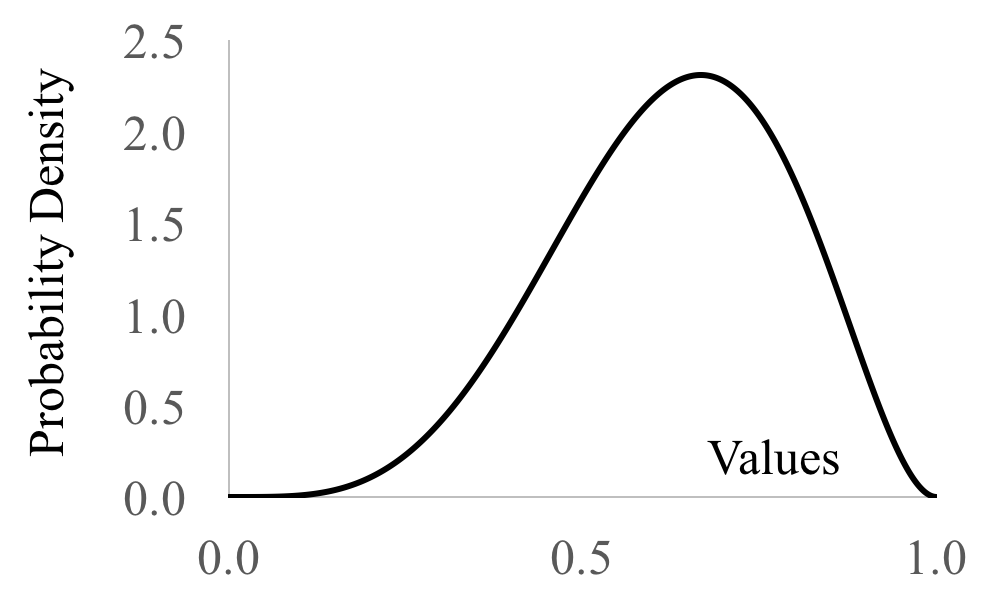
Notice how the most likely belief for the probability of curing a patient, is $4/6$, the fraction of patients cured. This distribution shows that we hold a non-zero belief that the probability could be something other than $4/6$. It is unlikely that the probability is 0.01 or 0.09, but reasonably likely that it could be 0.5.

Beta as a Prior

You can set $X \sim \Beta(a, b)$ as a prior to reflect how biased you think the coin is apriori to flipping it. This is a subjective judgment that represent $a+b- 2$ "imaginary" trials with $a-1$ heads and $b-1$ tails. If you then observe $h + t$ real trials with $h$ heads you can update your belief. Your new belief would be, $X \sim \Beta(a+h, b+t)$. Using the prior $\Beta(1,1) = \Uni(0, 1)$ is the same as saying we haven't seen any "imaginary" trials, so apriori we know nothing about the coin. Here is the proof for the distribution of $X$ when the prior was a Beta too:

If our prior belief is $X \sim \Beta(a, b)$, then our posterior is $\Beta(a+h, b+t)$: \begin{align*} f(&X = x|H =h, T=t) \\ &= \frac{P(H =h, T=t|X=x)f(X=x)}{P(H =h, T=t)} && \text{Bayes Theorem}\\ &= \frac{ { {h+t} \choose h} x^h(1-x)^t \cdot \frac{1}{c} \cdot x^{a-1}(1-x)^{b-1} } {P(H =h, T=t)} && \text{Beta PMF, Uniform PDF}\\ &= K \cdot x^h(1-x)^t \cdot x^{a-1}(1-x)^{b-1} && \text{Combine Constants}\\ &= K \cdot x^{a+h-1}(1-x)^{b+t-1} && \text{Combine Like Bases}\\ \end{align*} Which is the PDF of $\Beta(a+h, b+t)$

It is pretty convenient that if we have a Beta prior belief, then our posterior belief is also Beta. This makes Betas especially convenient to work with, in code and in proof, if there are many updates that you will make to your belief over time. This property where the type of distribution is the same before and after an observation is called a conjugate prior.

Quick question: Are you allowed to just make up priors and imaginary trials? Some folks think that is fine (they are called Bayesians) and some folks think that you shouldn't make up prior beliefs (they are called frequentists). In general, for small data it can make you much better at making predictions if you are able to come up with a good prior belief.

Observation: There is a deep connection between the beta-prior and the uniform-prior (which we used initially). It turns out that $\Beta(1,1) = \Uni(0,1)$. Recall that $\Beta(1,1)$ means 0 imaginary heads and 0 imaginary tails.